The fundamental approach of all impedance methods is to apply a small-amplitude sinusoidal excitation signal to the system under investigation and measure the response, which can be current, voltage, or another signal of interest¹. A typical i-V curve for a theoretical electrochemical system is shown in Figure 1.

¹ For example, in the case of Electrohydrodynamic (EHD) impedance spectroscopy, the signal is the rotation speed of the working electrode.

In potentiostatic EIS, a low amplitude sine wave ∆E ⋅ sin(𝜔𝑡) of a particular frequency 𝜔, is superimposed on the DC polarization voltage E₀. This results in a current response of a sine wave superimposed on the DC current Δi ⋅ sin(𝜔𝑡 + 𝜙). The current response is shifted with respect to the applied potential (Figure 2).

The Taylor series expansion for the current is given by:

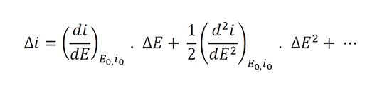
If the magnitude of the perturbing signal ∆E is small, then the response can be considered linear in the first approximation. The higher order terms in the Taylor series can be assumed to be negligible. The impedance of the system Z_ω can then be calculated using Ohm’s law as follows:

The impedance of the system is a complex quantity with a magnitude and a phase shift which depend on the frequency of the signal. Therefore, by varying the frequency of the applied signal, one can calculate the impedance of the system as a function of frequency. Typically, a frequency range of 100 kHz to 0.1 Hz is used in electrochemistry.

As mentioned above, the impedance is a complex quantity and can be represented in Cartesian as well as polar coordinates. In polar coordinates, the impedance of the data is represented by:

where |Z| is the magnitude of the impedance and 𝜑 is the phase shift.

In Cartesian coordinates, the impedance is given by:

where z' is the real part of the impedance, z'' is the imaginary part, and j = √(-1).

The plot of the real part of impedance against the imaginary part gives a so-called Nyquist Plot, as shown in Figure 3.

The advantage of the Nyquist plot is that it gives a quick overview of the data, and it is possible to make some qualitative interpretations. In a Nyquist plot, the real axis must be equal to the imaginary axis (i.e., isometric axes) so as not to distort the shape of the curve. The shape of the curve is important in order to make qualitative interpretations of the data. The disadvantage of the Nyquist plot is that the frequency information is not present. One way of overcoming this issue is by labeling some frequencies on the curve, as was done in Figure 3.

The impedance modulus and the phase shift are plotted as a function of frequency in two different plots collectively known as the Bode plot, shown in Figure 4. This is a more complete way of presenting the data.

The relationship between the two ways of representing the data is given by:

Alternatively, the real and imaginary components can be obtained from the following equations:

An introduction to electrochemical impedance spectroscopy (EIS) is given in this Application Note. The basic principles of how the impedance is calculated from the oscillating signals are discussed.

Additionally, the Cartesian and polar coordinates to write a complex number, together with the Nyquist plot, Bode plot, and 3D representation of the data are given.